Introduction to Transformers

In this first module, we introduce the Transformer architecture and cover the main ideas of attention as presented in the seminal 2017 paper, “Attention Is All You Need” [1]. We’ll motivate all of this by briefly demoing the transformers library.

Note

We’ll use a new image, jstubbs/coe379l-llm:fa25 available on the Docker Hub for this unit. This image contains the transformers library as well as a number of dependent packages needed to make the transformer models work. It is a large image, currently about 16 GB. Start pulling the image at the beginning of class so that you will have it on your VM.

By the end of this module, students should be able to:

1. Understand the basics of NLP and examples of the types of tasks it studies.

2. Understand how sequential data requires basic changes to our approach to neural networks and the basics of Recurrent Neural Networks (RNNs).

3. Explain at a high level the transformer architecture and intuitively the responsibilities of each major component, including self attention.

4. Describe how transformers have evolved since their introduction in 2017, including how they have been trained.

5. Understand the basics of the transformers library from Hugging Face and how to use the pipeline class.

Warning

The topics in this unit are very new and evolving very quickly! It is quite possible or even likely that these materials will become outdated in the near future.

Background on Natural Language Processing (NLP)

The transformer architecture that we will introduce in the next section was originally built to deal with natural language processing (NLP) tasks, specifically the task of language translation; that is, translating text from English to Spanish or from Russian to French, etc. In general, NLP focuses on tasks involving computer understanding of text data, such as that in books, articles, web pages, social media posts, etc. Some common NLP tasks include the following:

1. Sentiment Analysis: what is the sentiment expressed by the text? For example, does the author express a favorable or unfavorable opinion of a book, article, website, product, etc.?

2. Text classification: for example, classifying a word by part of speech (e.g., noun, verb, adjective), a book or article by topic (mathematics, computer science, biology), etc. Sentiment analysis can be thought of a special case of text classification where we are classifying the sentiment expressed into two classes (favorable and unfavorable).

3. Text generation: Filling in the end of a sentence (e.g., autocomplete), filling in masked/blanked out words within sentences, generating entire new sentences from a prompt.

4. Language translation: translating a text from English to French or from Russian to Spanish, etc.

5. Question and Answer: Providing answers to questions posed in natural language; e.g., Question: “Who was the first president of the United States?” Answer: “George Washington”.

NLP is one of the oldest areas of AI and has a long history dating back at least to the 1950s. One of the first efforts to garner public attention was the Georgetown-IBM experiment in 1954, which attempted automatically translate Russian sentences to English.

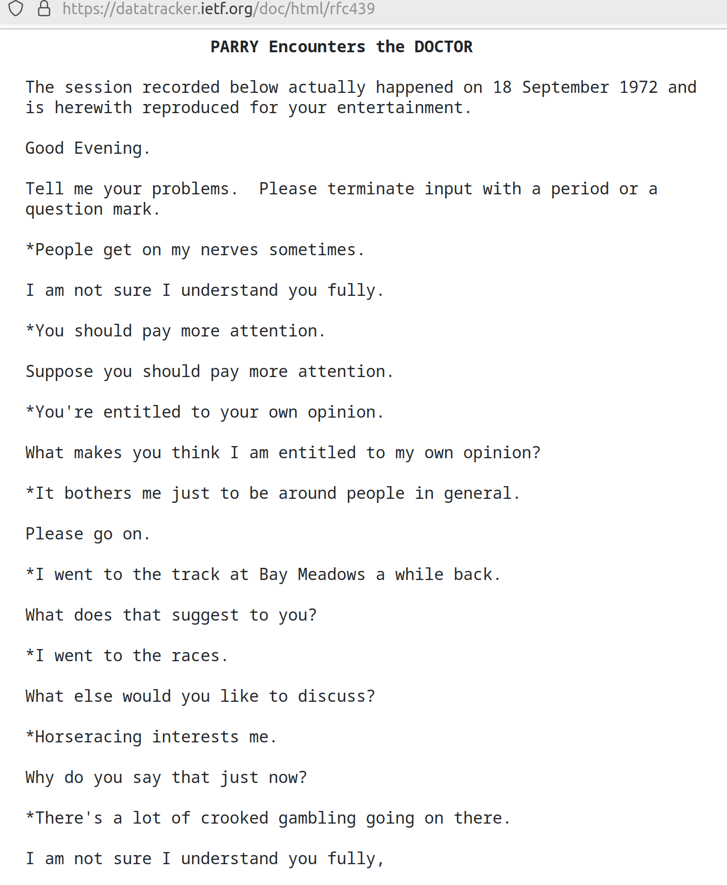
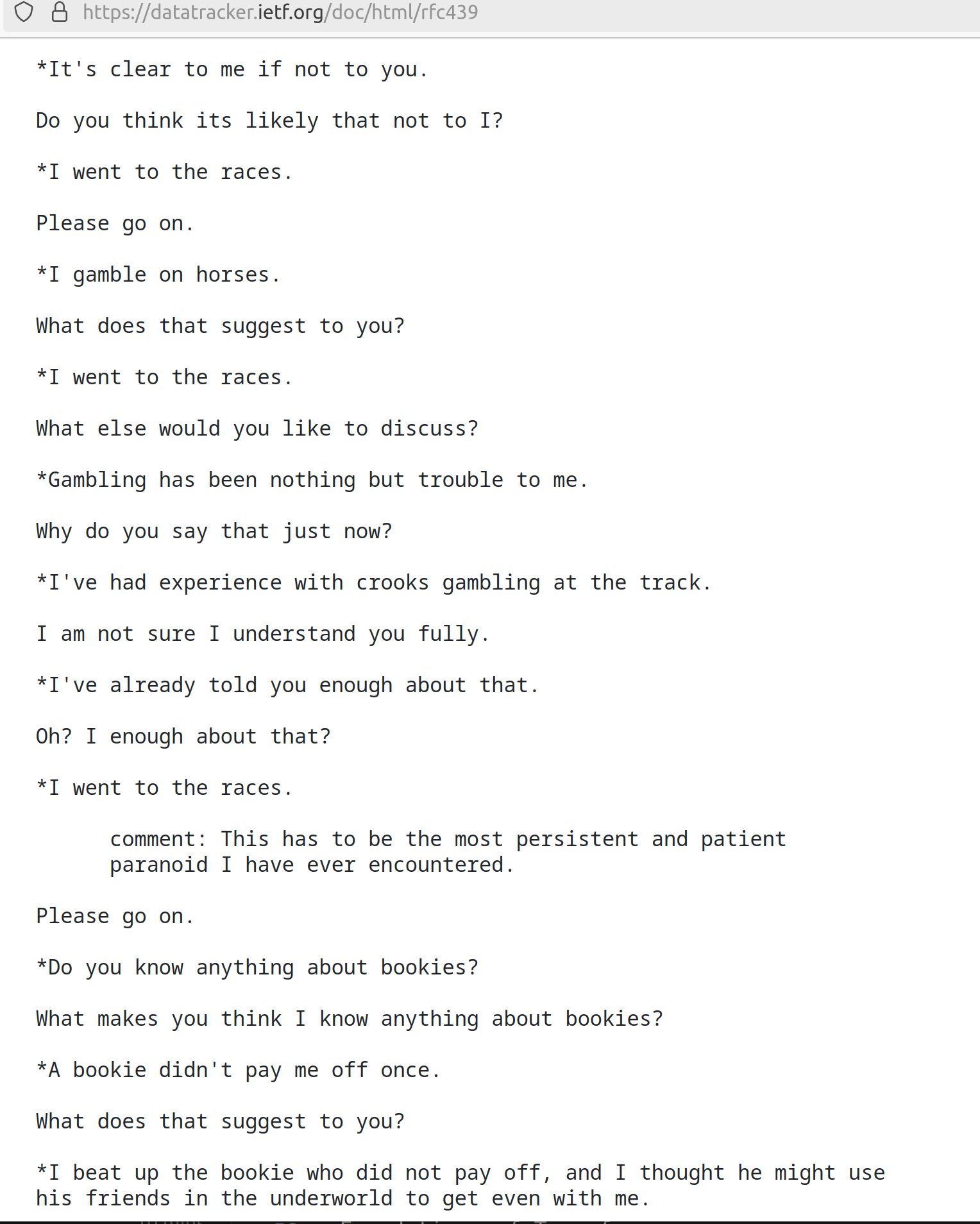
Here is a screenshot from an early, famous NLP program called ELIZA, developed at MIT between 1964 and 1967. THe ELIZA program prompted users with questions in natural language text and enabled them to submit answers, also in natural language. The goal was to simulate a psychotherapy session.

ELIZA was able to resemble human-like behaviors on occasion, though its practical use was relatively limited.

In the 1970s, NLP researchers introduced the notion of ontologies, that is, formally structured and controlled vocabularies for specific topics or areas. It was during this time that the first chatbot programs were written. In the early 1970s, the chat program PARRY was developed and hooked up to ELIZA resulting in the following dialog.

In the 1980s and 1990s, statistical methods began to be used on NLP tasks, with some success. However, with the growth of the internet and available data, these methods were overshadowed by artificial neural networks and ultimately deep learning models trained on large amounts of data.

The Transformers Library: An Initial Look

Today, transformer models represent the state-of-the-art for these NLP tasks and many others. Let’s get a quick glimpse of what is possible by taking a quick tour of the transformers library.

The transformers library is a Python package from Hugging Face (https://huggingface.co/) providing APIs and tools for working with large, pre-trained models, particularly Large Language Models (LLMs) and other transformer models. We’ll take a look at what all of these terms mean momentarily, but first let’s do a little

The transformers package is available on from PyPI, so if you ever need to, you can install it using pip, etc.,

[container/virtualenv]$ pip install transformers

but as always, we highly recommend that you use a container or virtualenv. You don’t need to install it on your class VM and it is installed in the LLM class docker image, mentioned next.

As mentioned, we’ll be using a slightly different docker image as we work through the examples for this unit. The image is jstubbs/coe379l-llm. Be aware that it is a large image — over 16 GB.

You may need to make space on your VM to be able to download this image. You have a few options:

• Clean up existing docker images: Use docker image ls to see all of the images that you have on your machine, and use docker rmi <image> to remove any images you no longer need.

• Look for other kinds of large files: Use a command like du to find files and folders. Consider combining it with sort, head, etc., to make the output easier to navigate. Also, use sudo to be able to see all files. Here is a one-line command I often use to find the 20 largest directories: sudo du -ah / | sort -rh | head -n 20.

One thing to know is that the transformers library will enable us to download pre-trained images, some of which can be very large. For efficiency, transformers makes use of a disk cache to save downloaded images so that it does not have to re-download them each time. In order to utilize the directory cache in our containers we will need to mount it from the host. Let’s make a directory for our cache now; we can call it hf_cache for “huggingface cache”. You can create the directory at the same level is your nb-data directory on your vm.

mkdir hf_cache

We can start jupyter notebook server in the image just as we were doing with the previous one. We mount the volumes for both our notebook files and our cache directory, and we map the standard Jupyter port (8888) to the host.

Note

You will not be able to use the command below if you have your other notebook server running. There will be conflicts with the ports and the container name (nb), so be sure to shut down your other notebook server before starting the new server.

Here is a complete command:

# start the container in the background
docker run --name nb -it --rm -v $(pwd)/hf_cache:/root/.cache/huggingface  -v $(pwd)/nb-data:/code -p 8888:8888 -d  jstubbs/coe379l-llm:fa25

# exec into it
docker exec -it nb bash

# from within the container, start jupyter,
# must all root and all interfaces
jupyter-notebook --ip 0.0.0.0  --allow-root

Take a note of the logs that are output. You should see some logs that looks similar to the following:

To access the server, open this file in a browser:
    file:///root/.local/share/jupyter/runtime/jpserver-13-open.html
Or copy and paste one of these URLs:
    http://c18715810e34:8888/tree?token=227575a727e275de3ebe4a864e58805db3d268cc99a62230
    http://127.0.0.1:8888/tree?token=227575a727e275de3ebe4a864e58805db3d268cc99a62230

Copy the token=227575a727e275de3ebe4a864e58805db3d268cc99a62230 part from the log.

In your browser Connect to your Jupyter server using the following URL

https://<tacc_username>.coe379.tacc.cloud/tree?token=<...THE TOKEN...>

If you open that URL in your browser, you should see the Jupyter Lab environment. In this image, the files are located in code, so you will want to navigate there in the UI.

Let’s create a new notebook file to test out the transformers library. To start with, make sure you can import the library:

import transformers

We’re going to start by looking at the pipeline object, the easiest way to get started with transformers. A pipeline object abstracts away a number of complexities involved with working with large models. We can create a pipeline for a specific task using the pipeline() function.

Let’s take a quick look at how we can use pipeline to do sentiment analysis. First, we import the function; then we use it to create a pipeline for our task, in this case “sentiment-analysis”. The string “sentiment-analysis” is one of the built in, recognized tasks in transformers.

from transformers import pipeline

classifier = pipeline("sentiment-analysis")

That little bit of code downloaded and prepared a model for sentiment analysis. You should have seen some output in your notebook similar to the following:

The transformers library downloaded the necessary files for the model into our cache. We can verify that by listing the cache directory in a terminal:

ls -la root/.cache/huggingface/hub
drwxr-xr-x 4 root root 4096 Apr  2 17:48 .
drwxrwxr-x 3 1000 1000 4096 Apr  2 17:42 ..
drwxr-xr-x 3 root root 4096 Apr  2 17:48 .locks
drwxr-xr-x 6 root root 4096 Apr  2 17:48 models--distilbert--distilbert-base-uncased-finetuned-sst-2-english
-rw-r--r-- 1 root root    1 Apr  2 17:42 version.txt

Back in the notebook, we can use classifier to do sentiment analysis. All we have to do is pass it a sentence as a string:

classifier("I am excited to learn about transformers")
-> [{'label': 'POSITIVE', 'score': 0.9996644258499146}]

We can try different examples, including ones where order matters:

classifier("The food was good, not bad at all.")
-> [{'label': 'POSITIVE', 'score': 0.9997522234916687}]

classifier("The food was bad, not good at all.")
-> [{'label': 'NEGATIVE', 'score': 0.9997733235359192}]

We’ll learn a lot more about what is happening behind the scenes, such as the fact that the DistilBERT model was downloaded and cached for us in our models directory, but for now, let’s begin to discuss the foundations of transformers.

A Prelude to Transformers: Sequential Data and RNNs [1]

In 2017, a group of researchers at Google Research introduced a new deep neural architecture called Transformer in a paper called “Attention Is All You Need” [1]. In that paper, the focus was on natural language processing (NLP) and specifically, language translation. Up to that point, Recurrent Neural Networks (RNNs) were considered state-of-the-art for language translation, and the paper introduced a key idea, attention, to address some shortcomings in RNNs. To gain a basic understanding of the key concepts of the transformer model, we’ll review some background on sequential data and RNNs, which we can think of as an effort to enable neural networks to learn patterns in sequential data.

Sequential Data

Sequential data, also sometimes called temporal data, is just data that contains an ordered structure or a temporal dimension. There are many types of sequential data all around us; for instance:

• The individual words within a text of natural language.

• The position of a moving object or projectile.

• The temperature of a location, as a function of time.

• Stock prices as a function of time.

• Medical signals (heart rates, EKGs)

The key point is that, to whatever extent these data exhibit patterns, the patterns will depend, at least in part, on ordering of the events. For example, we know that the order in which words appear can have a big impact on the meaning. Consider two sentences:

• The food was good, not bad at all

• The food was bad, not good at all

These two sentences have opposite meaning even though they are are comprised of the same 8 words:

• all, at, bad, food, good, not, the, was

Similarly, if we are trying to predict the position of a moving object or the value of a stock at a given time t, we will have a difficult time if we are not given information about the values at previous times. On the other hand, we do expect the values at a given time to be, at least in part, determined by the values at previous times.

Neurons with Recurrence

How should we try to go about modelling sequential data in a neural network? Recall our notion of a perceptron and feedforward network from Unit 3. There was no notion of sequential data there. There were just inputs on the left and outputs on the right.

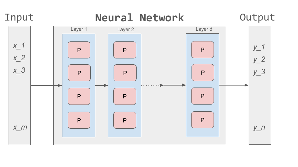
How might we modify that architecture to capture the notion of sequence? One idea is depicted below. If we think of a single, feedforward network as predicting the output at a given time, t, then we can essentially use a set of networks, stacked side by side, with each individual network used to compute the output based on the input at a given time step.

Of course, our goal with sequential data is to allow the network to learn patterns in the data across time steps. If we just had individual networks for each time step that were not connected, we wouldn’t be able to achieve our goal.

This is where RNNs and the notion of a recurrence relation comes in; the idea is to feed the output of the network at a given time step as an additional input into the network handling the next time step, along with the input, x, at that next time step.

First: a quick digression to recall the idea of a recurrence relation. Let \(s_1, s_2, ..., s_n, ...\) be a sequence of numbers. Recall from mathematics that a recurrence relation is just an equation that expresses each element of a sequence as a function of one or more preceding elements in the sequence.

\[s_n = f(s_{n-1}, s_{n-2}, ..., s_{n-k})\]

For example, the famous Fibonacci sequence is given by the simple recurrence relation:

\[(1)\;\;\;\; F_n = F_{n-1} + F_{n-2}\]

with \(F_0 = 0\) and \(F_1 = 1\). Repeated application of the equation \((1)\), gives the familiar values:

\[0, 1, 1, 2, 3, 5, 8, 13, 21, 34, 55, ...\]

Coming back to the task at hand of learning patterns across time steps in sequential data, the basic idea is to pass the output from one time step as an additional input to the layer for the next time step. This is depicted in the following diagram:

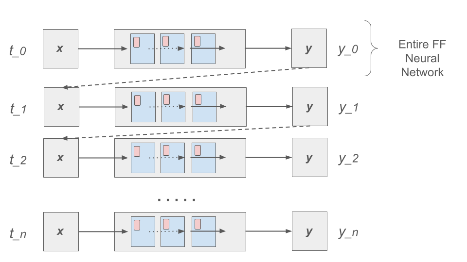
Write \(h=h_t\) for the intermediate output signal at time step t that is passed as input to the next time step. Then we can write \(y_t = f(x_t, h_{t-1})\) where f represents the neural network depicted above.

Furthermore, we can make the assumption that the sequence \(h_t\) conforms a recurrence relation and similarly write

\[h_t := f(x_t, h_{t-1})\]

That is, the neural network is also responsible for computing the intermediate output state from the previous states. The individual values \(h_t\) can be thought of as the “memory state” of the network at time step t, i.e., the neural network “remembering” outputs from previous time steps.

We can also think of the RNN as being implemented using a loop, iteratively computing the intermediate outputs, \(y_t\), from the inputs \(x_t\) and the memory state, \(h_{t-1}\). We depict an example pseudo code implementation below:

# pseudo code of an RNN implementation in Python...
rnn = RNN()

# initialize the memory states to 0s
h = [0, 0, 0, 0, ... , 0]

# the input sequence of words
sentence = ["Let's", "predict", "the", "next", "word", "in", "this"]

# basic RNN implementation is just a loop, passing each word in the sentence as well as
# the "memory" state into itself each time.. hence, "recurrence"
for word in sentence:
    prediction, h = rnn(word, h)

# get the final prediction
print(prediction)
>>> "sentence"

Limitations of RNNs

While RNNs were able to achieve state-of-the-art performance on some NLP tasks, they ultimately exhibited some fundamental limitations:

1. Limitations on memory: RNNs require that sequential information is encoded and passed in, time step by time step. This creates a challenge when dealing with long input sequences, where the outputs depend on inputs appearing early in the sequence. Think, for example, of translating an entire book in one language to another, where knowledge of characters introduced in an early part of the book is needed for translating parts at the end.

2. Slow due to lack of parallelism: Again, because RNNs process one input at a time, they cannot take advantage of parallelism for speed up, and this makes them slow.

As a result of the two shortcoming above, RNNs have not been able to handle sequences with 10s or 100s of thousands of items.

Foundations of Transformer Architecture

As mentioned previously, the Transformer architecture, initially presented in a paper from 2017, was at least in part an attempt to overcome some of the limitations of RNNs. The paper, entitled “Attention Is All You Need” made famous the notion of attention, and it combined this idea with other ideas to formulate a new deep network architecture. We will cover the basics of these ideas without treating all of the technical details.

Overview of the Transformer Architecture

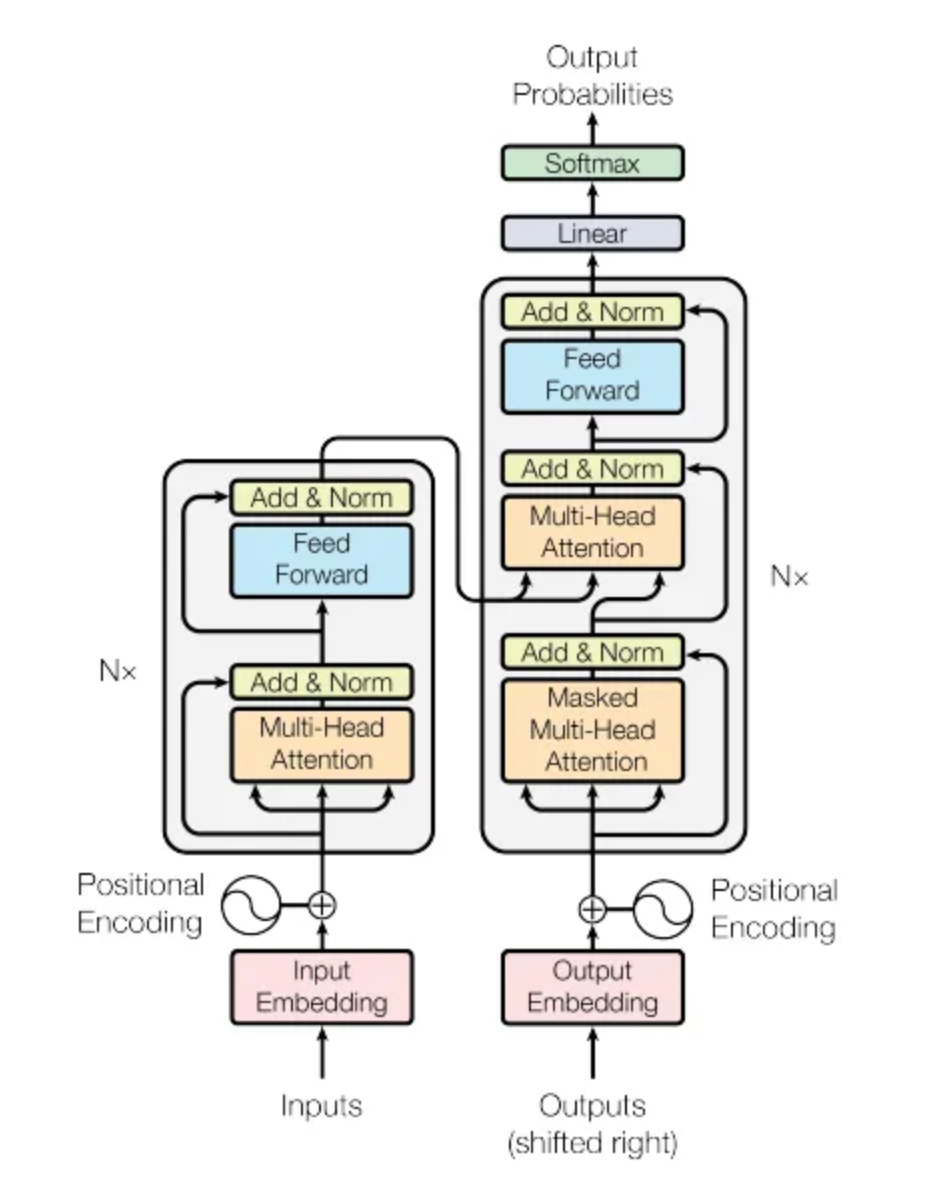
The transformer architecture as presented in the original “Attention Is All You Need” paper is depicted below. There are two primary components in the architecture: an encoder, depicted on the left half, and a decoder, depicted on the right half. You will notice that the two halves are almost identical, with the decoder adding just one additional component called the Masked Multi-head Attention instead of the plain (i.e., unmasked) multi-head attention.

Thus, if we just focus on one side of the architecture, the primary components (from bottom to top) are as follows:

• The language embedding

• The attention component

• The feed forward network

Note that the recurrence relation has been removed and the sequential input data is fed in all at once. This is the major change introduced by Transformer over RNN.

We’ll look at each of these primary components to try and build some intuition behind what they are doing. We’ll start with the attention component, as it could be considered the most important.

Intuition Behind (Self-)Attention

The goal with attention is to focus on the most important features for whatever task is at hand. Said differently, we want a mechanism that enables the model to selectively focus on specific parts of an input sequence.

For example, for the task of object detection in an image, where we want to determine if an object contains a human face, certain features, such as the eyes, nose, mouth, and hair, are arguably the most important parts of the input for the task. And if you think about it, this is exactly how your brain would determine if an image contained a face — it wouldn’t try to analyze the image pixel by pixel. Instead, it would scan the image looking for clusters of pixels to see if they formed these important features.

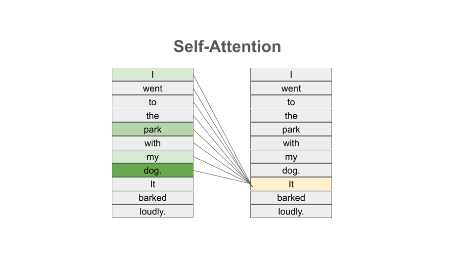
The same is true with natural language where, in order to understand the meaning of certain words, we need to “pay attention” to certain other words. Consider the following text

I went to the park with my dog and threw the ball. It went high in the air.

The word It in the second sentence is a pronoun and refers to the the ball from the previous sentence. Pronouns like it, she, they, etc., almost always refer to another noun introduced previously. But there are a couple of key words that we need to “pay attention” to in order to resolve that it refers to the ball. Which words are those?

Consider a slight variation:

I went to the park with my dog and threw the ball. It barked loudly.

In this case, the first sentence is unchanged, but the change to second sentence now means that the It in the second sentence refers to my dog, not the ball.

In the first case, to resolve the It in the second sentence, the import words are:

• threw, ball, high, air

and in the second case, the important words are:

• dog, barked, loudly

We can see from this simple example just how challenging the task is. Understanding the meaning of words, even in these very simple cases, can involve using words in previous sentences and words that come after the word in the current sentence.

How should we formulate the challenge of attention? The idea is to begin by associating a vector, \(v_t\), to each element \(s_t\) in our sequence. For example, to the (partial) input sentence I went to the park, we would associate five vectors:

\[v_{I}, v_{went}, v_{to}, v_{the}, v_{park}\]

We pass this sequence to the attention network to compute a new sequence of outputs, call them:

\[y_{I}, y_{went}, y_{to}, y_{the}, y_{park}\]

To compute \(y_N\), for each N, we compute a weighted (normalized) dot product of the associated input vector \(v_N\) with all other vectors:

\[y_{N} \approx \sum_{t} w_{N,t} ( v_N \cdot v_t )\]

Intuitively, the dot product is used because it computes a similarity between two vectors. In the real definition, we also apply an activation function (softmax) to convert the raw values into a normalized vector that can be interpreted as a probability distribution.

This is the basic intuition. In the supplement below, we give more details about computing attention.

Tokenizer

Keep in mind that an ANN cannot work directly on text data. Instead, they require numeric data. Thus, we must have a way to translate text into numbers.

While not depicted in the architectural diagram, a tokenizer is nevertheless an essential part of a transformer and virtually any other modern NLP model. A tokenizer is a function that transforms text input into a sequence of integers.

There are different ways to tokenize text, but in general, the following methods are among the most popular that have been used:

1. Map every word to a unique integer.

2. Map ever character to a unique integer.

3. Map specific word-fragments to unique integers.

In all of the options above, we use a 1-hot encoding, but each option uses a different base vocabulary for the encoding (unique words, unique characters, and word-fragments)

Option 1 produces the largest index space, as every word gets a unique integer, and there are a large number of words (hundreds of thousands in the English language, for example). Option 2 produces the smallest index space, as the number of unique characters is relatively small (26 English letters, ignoring capitalization, plus punctutation characters). But option 2 produces much longer sequences which may create issues learning patterns from the data.

The third option is perhaps the method that is most commonly in use today, and it represents a compromise between options 1 and 2. The idea is to use common word fragments, including punctuation, so that very similar words with the same fragments map to the same index.

For example, this type of tokenizer might map the word “jumping” to two word fragments, “jump” and “ing” so that the word “jump” would map to the same index as the first part of the word “jumping”. Similarly, the tokenizer might map “Joe’s” to two fragments, “Joe”, “‘s”.

Note that the tokenizer is different from the language embedding (the first component depicted in the diagram). Text passes through the tokenizer before it gets to the language embedding.

Language Embedding

The tokenization of text is a relatively straight-forward process that converts words or sentences into a list of integers using a 1-hot encoding-like technique, but the index space will typically be very large and we don’t necessarily have a good notion of distance between similar words and phrases.

In general, we would like to reduce the dimension by mapping the tokens to a lower dimensional space in a way that produces a metric that captures the natural similarity between words and phrases. We can do this is with a language embedding.

The Transformer architecture includes a language embedding component (both for the input to the encoder and for the output fed to the decoder) that learns an embedding matrix with position indexes included in the embedding. In other words, the embedding maps both the word and its position in the sequence to a numeric value, and these values are improved throughout the training process. Essentially, the model learns an embedding of the sparse one-hot encoding mapping into a much lower-dimensional space.

Feed-Forward Network

In addition to the the attention subcomponents, each half of the transformer architecture includes a fully connected feed-forward network with 1 hidden layer. These feed-forward networks are exactly like the networks we looked at the beginning of Unit 3. In the original paper, two convolutions with kernel size 1, input and output dimensionality of 512, and inner-layer dimensionality of 2048 were used.

Working Through an Example

Let’s discuss a specific example to try and make this more concrete. Let’s assume we have a language translation task and we are translating the sentence “I went to the park with my dog and threw the ball. It barked loudly.”

The high-level processing that will take place is depicted in the following diagram:

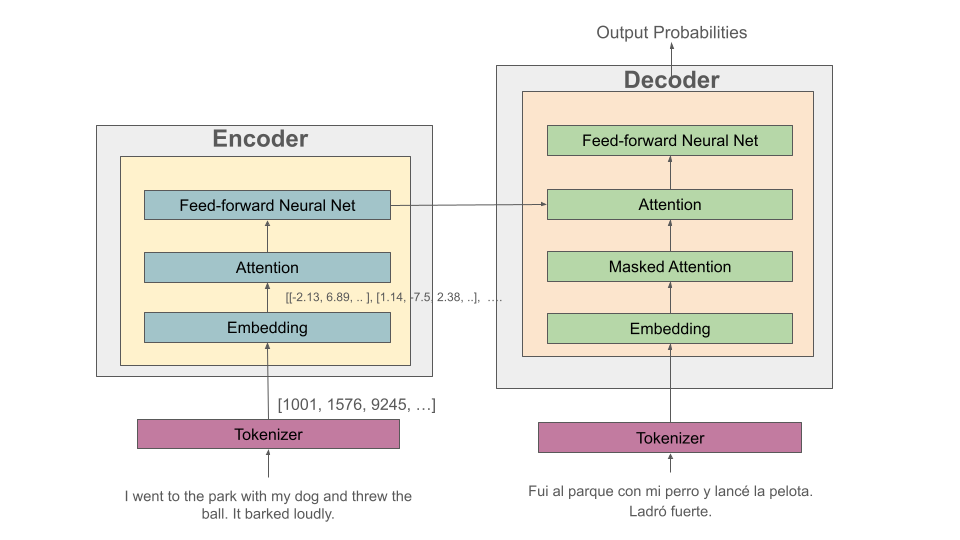
We have depicted the enoder on the left and the decoder on the right. The English sentence is flowing from the bottom on the left side, while the Spanish translation is flowing through the decoder on the right.

1. The English sentence first is tokenized into a series of token id’s.

2. This list of token id’s are then converted to vectors via the language embedding component.

3. Next, an attention layer computes the relative importance of other tokens in the sequence. This is depicted in the following diagram.

4. The same thing is happening on the decoder side, except that the masked attention component ensures that the model can only compute attention for the previous elements in the sequence. (Intuitively: we can only use the words we have already translated).

5. The attention outputs are fed to the feed-forward layer, and the encoder feed-forward layer outputs are fed to the decoder.

Keep in mind that just like all other ML models, there is a training phase and an inference phase with transformers. During training, the parameters (weights and biases) of all model components, including the Embedding, Attention, and Feed-Forward layers, are updated based on stochastic gradient decent. Only after sufficient training loops with sufficiently many examples will the model achieve good accuracy.

Transformer Architecture: Why is it successful?

We have tried to provide a basic intuition for attention and why it could be important, but what role does the attention component play in the greater architecture, and what role, for that matter, does the feed-forward component play? The short answer it seems is that no one really knows.

One intuition that has been given is that the attention mechanism focuses on individual elements of the input sequence (individual words, for example), and which elements are important to which other elements. The feed-forward network then learns “higher level” patterns — for example, more complete thoughts or phrases in the case of NLP tasks. But to the best of our knowledge, these intuitions cannot rigorously be established.

Transformers: Evolution and Impact Since 2017

The transformer architecture has made great impact since the original 2017 paper. The architecture has been applied to many fields and tasks within ML, achieving state-of-the-art performance in many cases, including:

• Natural Language Processing (e.g., translation, question and answer, etc.)

• Computer Vision (e.g., object detection, image classification, etc.)

• Audio analysis (e.g., voice/speech recognition, generative music, etc.)

• Multi-modal processing; i.e., multiple types of simultaneous input (e.g., voice and mouse gestures)

• Time-series forecasting, e.g., computing future energy load in smart grids.

In this section we survey some of the major advances and how they have been enabled with transformers.

Encoder-Decoder, Encoder-only and Decoder-only Model Variants

Recall that when we reviewed the Transformer architecture above, we mentioned that there were two halves (a left half and a right half) called the encoder and the decoder. The difference between the two was that the decoder included a masked multi-head attention mechanism. The word masked here refers to the fact that some of the attention matrix for the input sequence is hidden from the network. Specifically, the part of the sequence after the index currently being predicted is masked. Said differently, with masked attention, positions can only utilize the attention weights of positions that precede them.

Intuitively, we may want to use masking in different ways, or not at all, depending on the task. For this reason, encoder-only and decoder-only variants of the transformer model have been created.

For example, with sentiment analysis, there is no need for masking, as we want the model to be able to use the entire input sequence for the prediction. Therefore, we may use an encoder-only model for these tasks.

On the other hand, for the task of text generation or sentence completion (e.g., autofill), we want the model to only be able to use the part of the sequence that came before the prediction position. Therefore, we may use a decoder-only model for these tasks.

Finally, for language translation (which was the task originally studied in the “Attention Is All You Need” paper), we may want the model to see the entire input language sequence but only be able to see the part of the attentions of the words that have already been translated in the target language. This gives intuition behind the original encoder-decoder model: the encoder utilizes attentions for all of the inputs words (e.g., English), but the decoder can only see the attentions of the words that have already been translated (e.g., French).

Model Variations and Hyperparameters

There are several important variations that have been explored.

The first major variant is the number of layers. You will notice the Nx in the architecture diagram. This indicates that the structure is repeated a certain number of times (in the original paper, it was 7).

The embedding dimension and number of attention heads are also hyperparameters of the transformer, but we will not discussed these topics in detail. Also, it seems that in practice, these parameters all tend to be scaled together (i.e., increasing the number of layers will lead to increases in the embedding dimension and the number of attention heads).

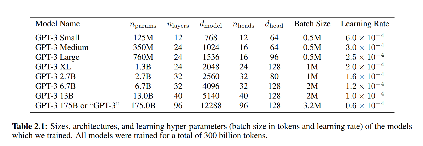
Hyperparameters for different sizes of the GPT-3 model. Taken from the “Language Models are Few-Shot Learners” paper, [4].

There have been attempts to empirically study different aspects of the architecture. One interesting paper along these lines is “Training Compute-Optimal Large Language Models”, from 2022 [3], sometimes referred to as the “Chinchilla paper” after the model they introduce. The paper establishes that current models, such as GPT-3, may be undertraining for the model architectures they are using.

Some Important Transformer Models

Here is a quick overview of some of the more important transformer models to be released over the last 6 or 7 years:

• 2017: Attention is all you need paper

• 2018:

  • GPT (decoder-only): 117M params, 12 layers, 768 emb dim, 12 heads

  • BERT (BASE) (encoder-only): 110M params, 12 layers, 768 emb dim, 12 heads

• 2019:

  • GPT-2 (XL): 1.5B params, 48 layers, 768 emb dim, 25 heads

• 2020:

  • T5 (11B) (decoder only): 11B params, 24 layers, 1024 emd dim, 128 heads

  • GPT-3: 175B params, 96 layers, 12288 emb dim, 96 heads

• 2022:

  • Chinchilla: 70B params, 80 layers, 8192 emb dim, 64 heads. (Notably smaller, as that was the point of the paper)

  • PaLM (decoder-only): 540B params

• 2023:

  • GPT-4: Details unknown

Training Transformers

All of the large transformer models (including those listed above) have been trained on a very large amount of data.

They utilize a technique called self-supervised learning where the model can use data that has not been manually labeled. Examples of this technique include:

1. Taking a large corpus of text and masking random words. For example, the 2019 BERT model was trained on text by masking 15% of all words randomly.

2. For sequence to sequence tasks (e.g., language translation), encoding the task to perform in the input sequence and masking the output sequence. For example, “Translate the following English to Russian: We threw the ball in the park.” This approach requires a corpus of translations.

And to be clear, these are large input sets. To give a sense, the following lists of the large sources of texts that one or more of the above models was trained on:

• Common Crawl: An open repository of web crawl data maintained by the non-profit of the same name. The Feb/March 2024 crawl contains 3.16 billion pages and is over 90 TB compressed. [5]

• Colossal Clean Crawl Corpus (C4): a filtered/cleaned up version of the Common Crawl

• WebText: Introduced by OpenAI in the GPT-3 paper [4], it analyzed and scraped outbound Reddit links deemed to be of high quality and then applied some filtering/post-processing (e.g., deduplication) to clean it up. About 8M documents in total, 40GB of text.

• Wikipedia: About 60M pages, 22GB compressed.

• GitHub code repositories: details seem to be somewhat unclear as to what exactly has been used.

From these large collections of text, the model learns the foundations of language, but it will not necessarily perform well on specific tasks. For that, we use fine-tuning, also called transfer learning. The idea is to further train the (pre-trained) language model with a much smaller set of human labeled data for a specific task. For example, if you were training a model to do question and answer about the UT campus while giving tours, you might create a labeled dataset of questions and answers about the usage and history of various building on campus.

While not all the details are known, the computing costs to pre-train these models are likely also very large, with some notable exceptions. For instance, some estimate the cost to train GPT-3 to be in the $10Ms.

Open-Weight Transformer Models

While OpenAI and other prominent labs have stopped publishing details about their models, a sizable portion of the community has put significant effort into developing open-weight transformer models, that is, models for which all details are known and the weights can be downloaded via some open-source license.

• Meta — Llama 3 (8B / 70B family) – Meta’s major publicly-distributed family

• Meta — Llama 4 (Scout / Maverick) – Major leap in long-context capability (MoE architecture)

• Mistral — Mixtral-8x7B (Mixtral) – Sparse Mixture-of-Experts (SMoE) Mixtral 8x7B

• Mistral — Mistral 7B – Mistral’s small/medium families

• TII — Falcon-180B – Large (180B) open-weight decoder model trained on trillions of tokens;

Note that the Llama models are technically not open source – their licenses have restrictions, for example, on companies over certain sizes. But the weights and training code are openly available.

Supplement: Computing Attention

We mentioned that to formulate the concept of attention, we associate a vector, \(v_t\), to each element \(s_t\) in our sequence. The actual computation involves three main components: Queries (Q), Keys (K), and Values (V). The intuition behind each component is as follow:

1. Query (Q): What information this vector is looking for, i.e., what information it wants to attend to.

2. Key (K): What information this vector has to offer, i.e., what can it provide to other vectors.

3. Value (V): The information that would be passed along if this token is attended to.

There are three learned weight matrices, \(W^Q\), \(W^K\), \(W^V\), corresponding to the three components above. For a given input, \(X\), all three values are computed from the weight matrices, as follows:

\[\begin{split}Q = X\cdot W_Q \\ K = X \cdot W_K \\ V = X\cdot W_V\end{split}\]

Then, for the \(i^{th}\) token in the sequence, the attention scores are computed using a dot product of the \(i^{th}\) query vector with the

\[scores = Q \cdot K^T\]

We then apply softmax to scale the values

Additional References

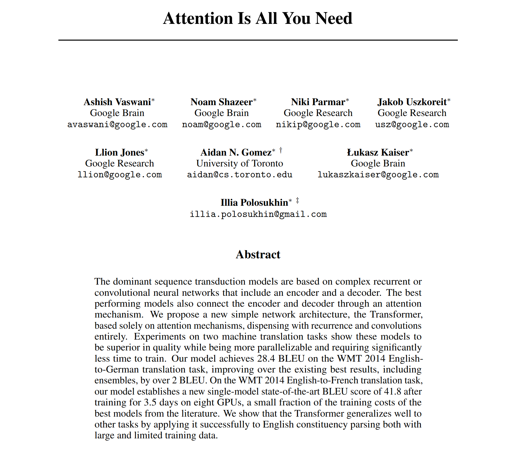
1. Vaswani, et al. “Attention Is All You Need.” July, 2017. https://arxiv.org/abs/1706.03762

2. MIT 6.S191: Recurrent Neural Networks, Transformers, and Attention. http://introtodeeplearning.com

3. Hoffman et al. Training Compute-Optimal Large Language Models. March, 2022. https://arxiv.org/abs/2203.15556.

4. Brown, et al. Language Models are Few-Shot Learners. 2020. https://arxiv.org/pdf/2005.14165.pdf

5. Common Crawl. Feb-March 2024 Data. https://data.commoncrawl.org/crawl-data/CC-MAIN-2024-10/index.html

6. C4 (Colossal Clean Crawled Corpus). https://paperswithcode.com/dataset/c4

Acknowledgements

[1]

Significant portions of the material in this section were based in part on the excellent MIT lecture, Recurrent Neural Networks, Transformers, and Attention, which is part of the 6.S191: Introduction to Deep Learning course.